
Cancer Diagnosis with Machine Learning
Problem Statement
Cancer is a complex disease that varies significantly across individuals, making accurate diagnosis and treatment challenging. Traditional diagnostic methods often struggle to account for the intricate variations in genetic mutations and the vast amount of clinical information in medical records. This project aims to address these challenges by leveraging machine learning models to predict cancer classes using both gene variations and textual data from clinical reports, thereby improving diagnostic accuracy and assisting oncologists in early detection and personalized treatment planning.
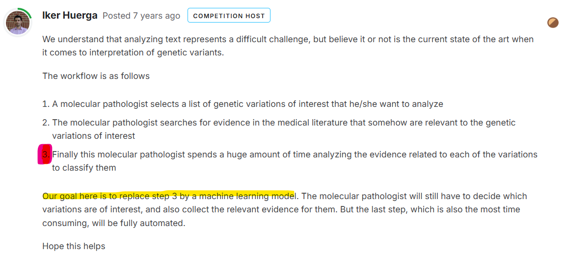
Figure 1: Problem Statement by Oncologist
Sources of Problem Statement
- Forbes: A New Cancer Drug Helped Almost Everyone Who Took It—Almost
- YouTube: Cancer Diagnosis Techniques (Video)
Business Constraints
- No low-latency requirement.
- Interpretability is important.
- Errors can be very costly.
- Probability of a data-point belonging to each class is needed.
Data Set Overview
- Source: Kaggle: MSK Redefining Cancer Treatment Data
- We have two data files:
- One contains information about genetic mutations.
- The other contains clinical evidence (text) used by experts/pathologists to classify these mutations.
- Both files share a common column called ID.
Data File Information:
- training_variants: (ID, Gene, Variations, Class)
- training_text: (ID, Text)
Data Preparation
Data preparation is a fundamental step in the machine learning workflow. It involves cleaning, transforming, and organizing data into a format suitable for modeling. Here, we will detail the preparation process for both the gene variation dataset and the text dataset.
1. Gene Variation Dataset
The gene variation dataset typically contains information on specific genetic mutations associated with different cancers. The preparation steps for this dataset include:
- Data Collection: In this project, we created a synthetic dataset that includes genetic information for several well-known cancer-related genes, such as BRCA1, BRCA2, TP53, EGFR, and KRAS. Each entry consists of the gene name, the specific mutation (variation), and a binary label indicating the presence or absence of a mutation.
- Data Cleaning: In a real-world scenario, this step would involve removing duplicates, handling missing values, and ensuring that the data types are consistent. Since our synthetic dataset is small and structured, it does not require extensive cleaning.
- Data Splitting: The dataset is divided into training and testing sets using an 80-20 split. This allows for the training of the model on one portion of the data while retaining another portion to evaluate its performance.
2. Text Dataset
The text dataset consists of clinical notes or research articles that discuss gene mutations and their links to cancer. The preparation steps for this dataset include:
- Text Collection: Similar to the gene dataset, we created a synthetic dataset that contains text entries related to cancer and genetic mutations. Each entry is associated with a label indicating the presence of a mutation.
- Text Preprocessing: Preprocessing involves several steps to clean and prepare text data:
- Tokenization: Splitting the text into individual words or phrases (tokens).
- Removing Punctuation and Stop Words: Eliminating common words (e.g., "and," "the") and punctuation that do not contribute significant meaning to the text.
- Lowercasing: Converting all text to lowercase to ensure uniformity.
Feature Extraction
1. TF-IDF Vectorizer
Using the `TfidfVectorizer`, we transform the text data into numerical features suitable for machine learning models. TF-IDF (Term Frequency-Inverse Document Frequency) is a statistical measure that reflects the importance of a word in a document relative to a collection of documents (corpus). By limiting the number of features to the top 1000 based on TF-IDF values, we reduce dimensionality and focus on the most relevant terms. This process involves:
- Tokenization: Splitting the text into individual tokens.
- Term Frequency Calculation: Evaluating how often a term appears in a document.
- Inverse Document Frequency Calculation: Determining the importance of the term across the entire corpus.
- Feature Selection: Selecting the top 1000 terms based on their TF-IDF scores.
2. BERT Pretrained Model
For an alternative approach, we leverage the power of BERT (Bidirectional Encoder Representations from Transformers), a state-of-the-art language model pre-trained on vast amounts of text data. BERT captures the contextual meaning of words within sentences, enabling more nuanced understanding and representation of text. When using BERT, the text data is transformed into features as follows:
- Tokenization: BERT requires a specific tokenization process that splits text into subword units.
- Input Representation: The tokenized input is converted into token IDs and includes attention masks to distinguish between padding and actual tokens.
- Feature Extraction: The BERT model outputs rich contextual embeddings for each token in the input, which can then be aggregated (e.g., using mean pooling) to obtain a fixed-size vector representation for the entire text input.
By utilizing these two different feature extraction techniques, we can explore various model performance levels and leverage the strengths of both traditional and modern approaches to text data.
Model Training
The model combines structured data (like genetic mutations) with unstructured textual information to improve classification accuracy. This involves steps like dataset preparation, feature extraction from gene variations and text, and the application of models like BERT for text, alongside traditional machine learning methods such as SVM, logistic regression, and neural networks for structured data. Performance is evaluated using standard metrics like accuracy/misclassification rate.
Results
| Model | Train Log Loss | CV Log Loss | Test Log Loss | Percentage Misclassification |
|---|---|---|---|---|
| Naive Bayes | 0.90 | 1.27 | 1.21 | 39.84% |
| kNN | 0.70 | 1.13 | 1.002 | 39.47% |
| Logistic Regression with class balance | 0.614 | 1.143 | 1.048 | 34.77% |
| Logistic Regression without class balance | 0.628 | 1.185 | 1.054 | 36.28% |
| SVM | 0.739 | 1.132 | 1.063 | 36.47% |
| BERT (base) | 0.10 | 0.13 | 0.18 | 12.43% |
Baseline: Log loss of a Random Model - 2.5